nnU-Net and TotalSegmentator

neural_flow draws nnU-Net v2 networks level by level and loads trained nnU-Net models straight from their results folders, with nnU-Net's own preprocessing, patch size, spacing and sliding-window settings. nnU-Net itself does not need to be installed; only the small dynamic-network-architectures package that nnU-Net builds its networks with.

The worked example is TotalSegmentator, whose public CT models are ordinary nnU-Net results folders.

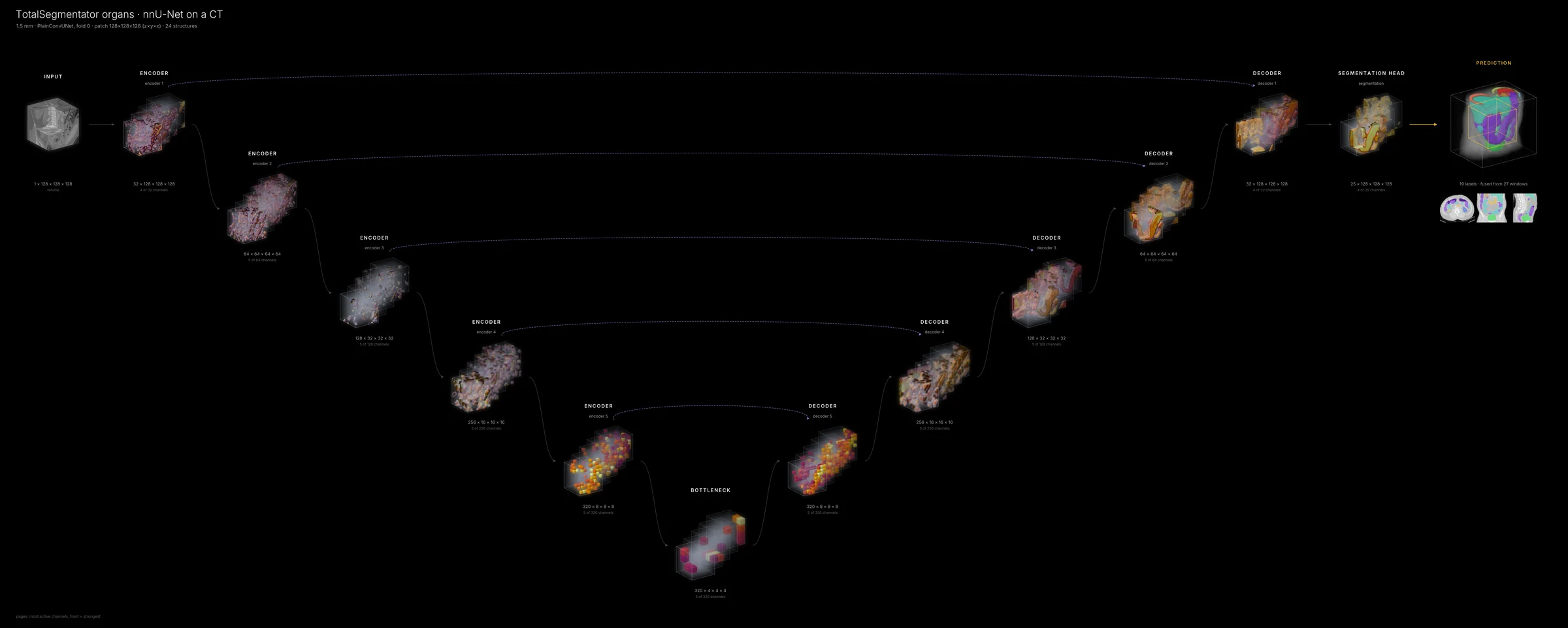
TotalSegmentator's 1.5 mm organ model (nnU-Net PlainConvUNet, 6 resolution levels, 24 structures) on its public example CT. Each encoder level bridges to the decoder level of the same resolution. The stages show one 128³ window; the output card is the whole CT fused from all 27 windows (the traced window is outlined), drawn to scale.

Quick start

pip install dynamic-network-architectures nibabel scipy     # or: pip install -e ".[medical]"
neural-flow fetch totalseg                                   # 3 mm model (≈135 MB) + example CT
neural-flow render totalseg -i sample:ct --sliding-window --style cinematic -o totalseg.png

neural-flow fetch totalseg-organs                            # 1.5 mm organ model (≈235 MB)
neural-flow render totalseg-organs -i sample:ct --sliding-window --style cinematic -o organs.png
neural-flow movie totalseg-organs --inference sample:ct -o organs_inference.mp4   # window by window

Your own trained model: point at its results folder, optionally with a fold (default 0):

neural-flow render nnunet:$nnUNet_results/Dataset123_Liver/nnUNetTrainer__nnUNetPlans__3d_fullres \
    -i case_0001.nii.gz --sliding-window --style cinematic
neural-flow render nnunet:$nnUNet_results/Dataset123_Liver:2 -i case.nii.gz --sliding-window   # fold 2, 3d_fullres picked
neural-flow inspect nnunet:$nnUNet_results/Dataset123_Liver -i case.nii.gz                   # the stages only

examples/nnunet_totalseg.py does the same in Python (both TotalSegmentator figures, --movie, and --results DIR --image CASE for your models).

What the figure shows

nnU-Net keeps each half of its U-Net in parallel lists that run interleaved: encoder.stages[i], and decoder.transpconvs[s] → concatenation with the skip → decoder.stages[s] → decoder.seg_layers[s]. The generic stage selection ran out of room inside those lists (upsampling layers but no decoder convolutions). The nnU-Net adapter recognises the layout by structure (no class names) and shows one stage per resolution level:

stage	module	concept
stem	encoder.stem (residual encoders only)	STEM
encoder 1 … n-1	encoder.stages[0 … n-2]	ENCODER
bottleneck	encoder.stages[n-1] (lowest resolution)	BOTTLENECK
decoder n-1 … 1	decoder.stages[0 … n-2]; the transposed convolution and the skip concatenation that feed it are folded into its incoming edges	DECODER
segmentation	the last decoder.seg_layers (full resolution)	SEGMENTATION HEAD

Decoder k rebuilds the resolution of encoder k, and the skip bridge joins the two. This works for PlainConvUNet, ResidualEncoderUNet (the nnU-Net ResEnc M/L/XL presets) and any other network with the same layout; neural-flow inspect prints the stages and skip edges it found.

Deep supervision. Networks built for training return a list of predictions, one per decoder level. As at nnU-Net inference, neural_flow sets deep_supervision = False while it runs the model (and restores it afterwards), so only the full-resolution prediction is drawn. aux_outputs=True keeps the auxiliary outputs.

Loading a results folder

nnunet:DIR[:FOLD] (or neural_flow.nnunet.load_nnunet(DIR) in Python) accepts the Trainer__Plans__configuration folder or its DatasetXXX_Name parent (3d_fullres is preferred, then 3d_cascade_fullres, 3d_lowres). It:

1. rebuilds the network from plans.json with dynamic_network_architectures, for the current plans format (architecture block) and the older one (UNet_class_name, used by TotalSegmentator v2);
2. loads fold_N/checkpoint_final.pth (else checkpoint_best.pth), with deep supervision off;
3. takes the class names from dataset.json (region-based models are loaded too; their outputs are independent sigmoid regions);
4. attaches nnU-Net's preprocessing and inference settings:

step	nnU-Net	neural_flow
reading	NibabelIOWithReorient / SimpleITK: RAS, axes reversed to [z, y, x]	the same; the figure uses volume_axes="zyx"
cropping	to the non-zero bounding box	the same (without hole filling)
normalisation	per channel from the plans (CTNormalization: clip to the 0.5–99.5 % foreground percentiles, then z-score with the dataset's mean and std; ZScoreNormalization …)	the same schemes
resampling	to the plans' spacing, cubic spline, separate z for very anisotropic scans	cubic spline via SciPy (trilinear without SciPy), no separate z
sliding window	plans' patch size, step 0.5, Gaussian σ = patch/8	the same (--sliding-window uses them automatically)
test-time mirroring, fold ensembles	on by default	not used (one fold, one pass)
export	back to the original geometry	the prediction stays in the network's space

The spacing drawn is the plans' target spacing, so the volumes have true proportions.

Checked against TotalSegmentator. On the example CT, the 3 mm model loaded this way agrees with TotalSegmentator's own reference segmentation: Dice 0.95–0.98 for spleen, kidneys, liver and stomach, and 97.7 % of the voxels identical. The reference was computed on a 30-slice crop of the same CT (example_ct_sm.nii.gz), so some differences near the crop edges are expected. tests/test_nnunet.py repeats this check whenever the weights are present.

Python

from neural_flow import visualize_model, zoo

lm = zoo.load_model("nnunet:/path/to/Dataset123_Liver/nnUNetTrainer__nnUNetPlans__3d_fullres")
info = {}
x = zoo.load_input("case.nii.gz", lm, info=info, whole=True)        # preprocessed [1, C, z, y, x]
visualize_model(lm.model, x, style="cinematic", sliding_window=True, roi_size=lm.roi,
                sw_overlap=lm.sw_overlap, volume_axes=lm.volume_axes, voxel_spacing=info["spacing"],
                class_names=lm.class_names, output_types={"output": "segmentation"}, output="liver.png")

A network you build yourself (for example nnUNetTrainer.build_network_architecture(...) or get_network_from_plans(...)) needs nothing special: pass it to visualize_model and the adapter does the rest.

Memory and time

The gradient explanations (the receptive-field circles and beams) need one backward pass through a whole patch. For nnU-Net's large 3-D patches this is several GB (neural_flow estimates about 5 GB for TotalSegmentator's 112×112×128 patch and 6 GB for 128³). It estimates the need first and skips the explanations with a note when they would not fit in 80 % of the free memory; on a machine with more memory, --set explain_max_mb=16000 forces them, and --no-explain always skips them. (The 3 mm gallery figure has explanations, forced with python examples/nnunet_totalseg.py --model totalseg --explain-max-mb 7000; the 1.5 mm one was rendered on an 8 GB machine without them.) The forward passes are light: on a laptop CPU the 3 mm figure takes about two minutes and the 1.5 mm organ figure (27 windows) about six.

References

Isensee et al., nnU-Net, Nature Methods 2021; Isensee et al., nnU-Net revisited, MICCAI 2024; Wasserthal et al., TotalSegmentator, Radiology: Artificial Intelligence 2023. Full entries: References.